I’ve just completed one more course of Pluralsight’s Data Science Foundation learning path: “Play-by-play: Machine Learning Exposed” by James Weaver and Katherine Beaumont. The course consists of three modules: Machine Learning introduction, supervised learning, and reinforcement learning.

In this post, I’ll focus on some important concepts and definitions of supervised learning, one of the three main types of machine learning. 

Introduction

Traditionally, developers have built programs that work in a prescribed way. Machine learning takes a different approach, one that mimics the human way of thinking. That is: learning by observing and by being taught. 

There are three main types of machine learning: 

• Supervised learning: you provide the algorithm (input) and the correct answers.
• Unsupervised learning: instead of providing the right answers, you just provide data, and the program tries to make sense of the data (for example: clustering algorithms)
• Reinforcement learning: you try to get an agent to learn something with an incentive, a “reward” if something is correctly analyzed. Example: AlphaGo contest -> https://deepmind.com/alphago-korea

Supervised Learning Concepts

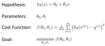
Let’s start by presenting some concepts that will be used very frequently in this context. The first one is hypothesis, which can be defined as a “proposal”. A hypothesis (also known as model) can be used to map inputs and outputs. Our hypothesis would be that the price of a house can be calculated based on its size.

The line that connects the dots where the price and the size of a house converge can be represented with this formula:

Y = MX + C

Where:

• C is the point where the line intercepts the y-axis (where the price starts)
• M is the gradient of the line (how steep it is). Gradient = rate of change = change in y / change in x

Theta (a cero with a line through it θ) is the “weight” of a function. In this case, it represents the M and C variables. The training data is used to define its value, which, in turn, can be used to make a prediction when feeding new data to the function. 

After a hypothesis is defined, we can make a guess. For example, if m=0.1 and c=0.7, y= 0.1x + 0.7.

With a guess in place, we now need to find a way to know how right or wrong this guess is. This can be achieved by drawing a line between the value of our guess and the real value, or between our prediction and the real price. The difference between the two values is the absolute error, or between h(x) and y.

Then, we can square the absolute error for each value, add them together and calculate the average over the number of examples. This concept is also known as the cost function.

Why do we square it? For two reasons: 

• To always obtain a positive number
• To increase the visibility of a trend by multiplying the values

If we take another guess (use different values for theta), we can compare the averages of the absolute errors and choose the one that is more accurate. We can keep taking guesses until we find the optimum value, which is the one that has the lowest absolute error average.

This is the point where the gradient is cero, because the cost function is flat.

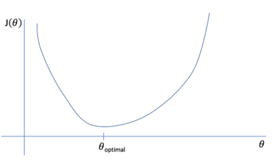
How can we optimize the process of finding the optimum value for theta? By using the gradient descent function. This function is a general function that can be used to minimize another function. In this case, the cost function.

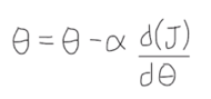
We use this function to adjust the value of theta by applying a learning rate (represented by alpha). The learning rate means how fast we want to move to the desired minimum or optimum value or how much are we going to change data each time. We have to be careful when defining the learning rate, as we can overshoot the optimum value if the learning rate is too large. 

If the cost function is increasing, the rate of change will be positive, so we need to reduce the learning rate. If it decreases, the rate of change will be negative, and we have to increase the value of the learning rate.

This function will help us to define a linear regression, which uses the relationship between variables to find the best fit line to make predictions. You can use it when there is a rough correlation between the variables. E.g. the bigger the house, the more it costs.

If the variable data is correlated but the relationship is not linear, we can use a polynomial linear regression.